Beyond "Area Under the Curve"

Other ways of thinking about definite integration. | July 14, 2025 | 2075 words, 11 min

In most textbooks, definite integration is described as the operator yielding the "area under the curve" of a given function. While the description is correct, thinking about integration only in terms of area is an oversimplification and can become a barrier to understanding why we use integration in other contexts, such as in determinations of volume and arc length. Thus, in this post, I'd like to discuss other ways of thinking about definite integration with the aim of facilitating a more intuitive understanding of definite integration.

1. Solids of Revolution

I want to begin by providing some background and a motivation for such an approach and will use a topic that I saw many classmates struggle with: rotational solids. A problem may ask,

Example 1.1: Determine the volume of the solid obtained by rotating the region bounded by $f(x)=x^2, x=1,x=3,$ and the $x$-axis, about the $x$-axis.

Figure 1 - Graph of $y=x^2$

If we view integrals as simply giving us the area under a given function, then developing an intuitive understanding of example (1.1) may not be obvious. Since integrals give us area, per the conventional definition, not volume, we can begin by finding a way to translate the 3-D problem into 2 dimensions. We start with the observation that rotating a single point $(x_i,y_i)$ on our graph about the $x$-axis would yield a circle of area $\pi y_i^2$. Therefore, to determine the volume $V$, we look for a function $g(x)$ that, at a point $x$, yields the area of a circle passing through $x$ and centered at point $(x,0)$ on the $x$-axis. Under the traditional definition, therefore, integrating $g(x)$ will yield the "area under the curve" of $g(x)$, which is the volume, $V$.

We can evaluate this expression using the antiderivative¹ of $x^4$:

The method in (1.1), while not intuitive, can be used to explain derivations of volume, but introduces complexities very quickly as we move to more advanced problems such as (1.2) below.

Example 1.2 (Take 1) Determine the volume of a solid whose base is the region contained by $y=(9-x^2)^{1/2}$,$x=1$, $x=3$, and $y=0$, and has cross-sections perpendicular to the $x$-axis that are equilateral triangles.

Figure 2a - Graph of $y=\sqrt{9-x^2}$ 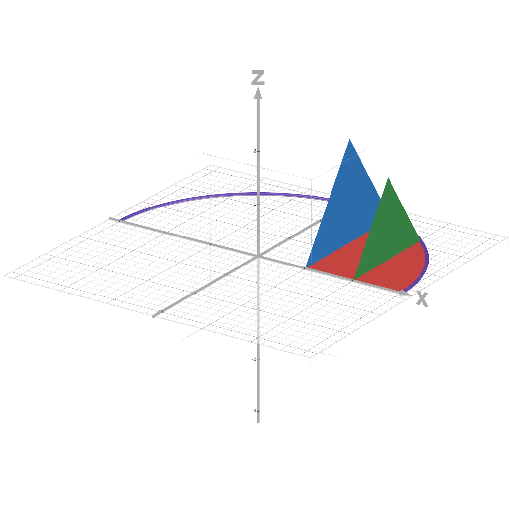Figure 2b - Graph of 2 equilateral triangle cross-sections for (1.2)

With (1.1), we translated our problem into 2 dimensions first. Let's do that again. Given any point on $y=\sqrt{9-x^2}$, the $y$-value becomes the length of the base of an equilateral triangle. So, we should integrate a function that gives us the area of these equilateral triangles. In the case of (1.2), that function would be $\frac{\sqrt 3}{4} s^2$, where $s$ becomes $y=\sqrt{9-x^2}$.

As we can see, examples such as (1.2) can get complex and non-intuitive very quickly. For example, one could change the boundary from $y=0$ to $y=10x$, and rotate about the $y$-axis, resulting in an even less intuitive problem. Although thinking about "area under the curve" works, constantly having to translate between 2-D and 3-D is a barrier to a deeper understanding.

2. An Intuitive Approach to Understanding Definite Integration

There exist other issues with the "area under the curve" definition that I've seen other students struggle with, which will be the focus of the rest of this post. Namely,

1. Why does the change in the antiderivative give us the area, and why is the antiderivate be related to area at all?
2. Why do we need a differential (e.g. $dx$) at the end of the integral?
3. Integration is also used for calculation of arc length. Since arc length leads to a seemingly arbitrary formula, the question arises, why do we use an integral, which should output area, to find the length of a curve?

Question (a):

The answer to our first question also gives us a new way of approaching integration.

Here's a visual example:

Here, we can see a linear function (Fig. 3a) and its antiderivative (Fig. 3b). More specifically, in Fig. 3, we are interested in the relationship between the area of the the function and the change in its antiderivative. We notice that the change in the antiderivative is very close to the sum of the heights of the boxes.

Visually, we can think about the diagram another way: the graph is of a quadratic function (on the right) and it's derivative (on the left). Now, the relationship between the functions makes more sense. The height at any one point on a derivative, $f'(x)$, is defined to be the instantaneous rate of change of $f(x)$. Conversely, the height at any one point on a function, $f'(x)$, must be the instantaneous rate of change of an antiderivative, $f(x)$. Therefore, for thinner and thinner boxes, the area of the function becomes closer to the actual change in the antiderivative! In other words, we are looking at the limit of the area of the function as $dx \to 0$.

Thus, the diagram leads us to a new way of thinking of integration. As $dx$ gets closer to 0, our integral beomes more and more like a sum. Therefore, we may think of the integral as a sum, which adds up a continuous set of values.

Question (b):

We can also approach the diagram algebraically, and answer the second question. Let's call the function on the left $f(x)$, and the width of each box $dx$. If we are trying to find the area of $f(x)$, we should sum up the areas of the boxes for a very small value of $dx$. In other words, we are adding up the values of $f(x) \times dx$ for each box. Also note, however, that $f(x)$ is the derivative of the function on the right, which we can call $y$, which means that we can write $dy/dx$ instead of $f(x)$. Therefore, the area is $\frac{dy}{dx} \times dx = dy$, added up for each $x$-value. If we write the expression in an integral as $f(x) dx$, then the $dx$ is "multiplied" by $f(x)$, and we can just measure the change in our antiderivative to calculuate the sum!

Our new definition means that we can also use integrals any time we try to add up a lot of different continuous values. Let's revisit the problem about solids of revolution:

Example 1.2 (Take 2) Determine the volume of a solid whose base is the region contained by $y=(9-x^2)^{1/2}$,$x=1$, $x=3$, and $y=0$, and has cross-sections perpendicular to the $x$-axis that are equilateral triangles.

Instead of thinking about finding a given function that gives the area of the cross-section, we can think about adding up the areas of equilateral triangles with side length $y$. The area of an equilateral triangle with side length $s$ is $\frac{\sqrt{3}}{4}s^2$, so we can write our integral as:

We are no longer looking at the area under the curve of a function. Instead, we are adding up all the values of the function at each point. Viewing integrals as a sum allows us to more intuitively understand its use in why we can use integrals in so many different contexts, such as when used to determine the average value of a function or the arc length of a curve.

3. Approaches to Problem Solving and Other Uses

The sum definition gives us a powerful tool for problem solving. Let's condense the methodology we applied in (1.2) into a set of steps we may follow when approaching a problem relating to integration:

1. Find what you are adding up, e.g a triangle, set of $y$-values, etc.
2. Find the range you are adding over, e.g. a range of $x$-values, $y$-values, or even a time interval. Keep in mind which variable you are changing, the variable will help you determine whether to integrate with respect to $dx$, $dt$, etc.
3. Take your function from step 1 and multiply it by the differential (e.g. $dx$, $dy$, etc.) from step 2, which yields the area of a rectangle, representing the change in your antiderivative.
4. Integrate the function and differential over the range from step 2, which bceomes your final answer!

Question (c):

We can apply the approach above to determine arc length as illustrated in (3.1):

Example 3.1: Find the length of $f(x)=\sin(x)$ from $x=0$ to $x=\pi$.

Let's try and follow our steps:

1. What are we adding up? In (3.1), we need to find the length of the curve, so we are adding up the lengths of little line segments along the curve. We know from algebra that the length of a line segment is $\sqrt{(\Delta x)^2 + (\Delta y)^2}$. We also know that $dx$ and $dy$ are the changes in $x$ and $y$, respectively, so we can rewrite the line segment as $\sqrt{(dx)^2 + (dy)^2}$.
2. Our range in (3.1) is from $x=0$ to $x=\pi$, so we will integrate from 0 to $\pi$, and our differential will be $dx$.
3. In (3.1), the differential $dx$ is already present in the function, so we can do a bit of algebra to rewrite our function. Keeping in mind that $dy = f\prime(x)dx$, we can write:

4. Now, we can integrate our result from Eq. 4 over 0 to $\pi$:

It is important to note that the manipulation of $dx$ and $dy$ that we performed in step 3 is frowned upon by mathematicians because there can be situations where we cannot treat $dx$ and $dy$ as variables. However, when embarking on a study of introductory calculus, the method provides a more intuitive approach to develop understanding of definite integration.

Conclusion

I hope this post has given you a new way of approaching definite integration. It is a powerful tool that can be used in many different contexts, and I believe that thinking of integration as a way to add up values rather than just finding the area under a curve will help you understand the applications better. I encourage you to explore some of these applications, such as in physics, economics, or in further math. If you want some practice, I recommend working through some integration bee problems.